Author Archives: Patrick Nixdorf

Stay at the cutting edge thanks to Packet Slicing

Slicing - Photo by Brands&People

Problem

Sling - Photo by Brands&People

Often the gap between the capacity of the recording analysis system on the one hand and the amount of incoming data on the other is so large that without appropriate additional mechanisms the analysis system is most likely not able to record all individual packets without loss.

Depending on the purpose of the analysis system, this is a major problem, as every packet counts, especially in the cyber security environment, and otherwise it is not possible to ensure that all attacks and their effects are detected.

Attacks that are not detected in time or even remain completely invisible can cause enormous damage to companies, even leading to recourse claims from possible insurers if they discover that their clients did not fulfil their duty of care.

But how does such a situation arise? It can happen very quickly that networks in companies grow, often in parallel with the business development of this company, while the often already existing analysis and monitoring systems, planned with reserves during procurement, reach the end of their reserves more and more often.
Higher bandwidths, more and more services and interfaces used in the LAN reduce the capacities to the point where the systems can no longer keep up and have to discard packets.
Photo by Lars Kienle
From this moment on, it is theoretically possible for an attacker to stay undetected in the local network, as the analysis system is hopelessly overloaded. The administrator is no longer able to see which parties in his network are talking to each other, which protocols they are using and which endpoints are being communicated with outside the LAN.

Often, however, it is not capacity problems that trigger the activation of Packet Slicing, but rather data protection reasons. Depending on where and which data is tapped and when, it may be obligatory for the company to only record and evaluate data that does not contain any personal or performance-related information.

While typically the packet header only contains connection data (WHEN, WHO, HOW, WHERE), the payload data, although usually encrypted, contains the very content data that theoretically makes it possible to measure the performance of individual users. Depending on the place of use, however, this is often neither wanted nor allowed. It must therefore be ensured that it is not possible for the administrator to reconstruct personal information from the recorded data.

Reduce analysis data by means of Packet Slicing

87 percent less thanks to Packet Slicing
And this is exactly where the “Packet Slicing” feature comes into play: with this procedure it is possible to reduce the incoming data load on your analysis system by up to 87% (with 1518 bytes packet size and Packet Slicing at 192 bytes) by simply removing the user data from each packet.

Many analysis and monitoring approaches only need the information stored in the packet header, i.e. the metadata, for their evaluations and analyses, while the user data often does not contain any important or usable information, as this is usually encrypted anyway and thus cannot be used for the evaluation.
By removing the user data, a massive relief of the processing instance is to be expected, and in some cases this enables even greater coverage of the LAN by the monitoring and analysis device.

FCS Checksum Problem


An important aspect of Packet Slicing is the recovery of the FCS checksum of each modified packet. Since the structure and length of the packet is affected by cutting away the user data, the originally calculated checksum, which was calculated by the sender and entered in the FCS field of the packet header, is no longer correct.

As soon as such a packet arrives on the analysis system, those packets are discarded or declared erroneous, as the checksum in the FCS field is still based on the original packet length. To counteract this, it is essential that the FCS checksum is recalculated and also entered for each packet from which the user data has been removed, as this would otherwise force the analysis systems to classify these packets as faulty and/or manipulated.

Network Packet Broker as a Packet Slicer

In general, there are several possibilities where the above-mentioned Packet Slicing can be activated in the visibility platform used by the customer. On the one hand, this is a case-by-case decision, on the other hand, it is also a technical one.

NEOXPacketLion - Network Packet Broker - Network Monitoring Switch | Data Monitoring Switch

Assuming that the user has set several measuring points distributed in his network, a Network Packet Brokeris often used. This device is another level of aggregation and is typically used as the last instance directly before the monitoring system. A Network Packet Broker is optically very close to a switch and enables the user to centrally combine the data from multiple measuring points (Network TAPs or SPAN ports) and send them aggregated in one or more data streams to the central analysis system.

Thus, for example, the data from 10 distributed measuring points set in 1 Gigabit lines can be sent to an analysis system with a single 10 Gigabit port by the Network Packet Broker aggregating these 1 Gigabit signals and outputting them again as a single 10 Gigabit signal.

NEOXPacketRaven Network TAP - OM4 to RJ45At this point, however, the user learns of a catch to the whole issue: often the analysis systems, although equipped with a 10Gigabit connection, are not able to process bandwidths of 10Gigabit/second as well.

This can have a variety of reasons, which, however, should not be the subject of this blog entry. However, the initial situation is predestined for the use of Packet Slicing; while one would normally have to expand one’s monitoring infrastructure at immense cost, by switching on Packet Slicing one can massively reduce the incoming flood of data and thus continue to use one’s existing systems; all that is needed is a corresponding instance with precisely this feature, which usually costs only a fraction of what would be estimated for an upgrade of the analysis systems.

Analysis Systems as Packet Slicers

Napatech High Performance Smart-NICsAnother possibility is offered to the user on the analysis systems themselves. Depending on the manufacturer, structure and components used, it is possible to directly remove the user data on the systems themselves and recalculate the checksum before the packets are passed on internally to the corresponding analysis modules.

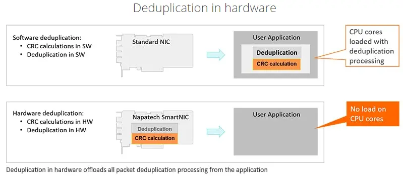
In the vast majority of cases, an FPGA-based network card is required for this, as it must be ensured that no CPU-based resource is used to modify each individual packet. Only by means of pure hardware capacities can the user be sure that every packet is really processed accordingly; any other approach could again lead to the errors and problems mentioned at the beginning.

Packet Slicing to meet Legal Requirements

Another aspect worth mentioning is the fulfilment of legal requirements. Especially in the context of the GDPR, it may be necessary to remove the user data, as often the metadata is sufficient for an analysis.

For example, if you want to analyse VoIP, you can use Packet Slicing to ensure that unauthorised persons cannot listen to the conversation, but you can still technically evaluate the voice transmission and examine it for quality-of-service features. This allows performance values to be evaluated, privacy to be protected and legal requirements such as the GDPR to be met.

Conclusion

So we see that there are indeed different ways to distribute the final load on the analysis and monitoring systems or even, as in this example, to reduce it without losing the most important information for creating performance charts, top talkers and more. Packet Slicing is therefore a valid solution for the user, which can be easily implemented in almost all cases and achieves usable results.

Use monitoring resources more effectively thanks to intelligent Load Balancing

Problem

Often, analysis, monitoring and security systems have more than one port to accept and process incoming data from the corresponding network access points. Many of these systems have at least 2, 4 or even more ports ready to accept data.

Depending on the type and location of the various network access points, this offers the user the option of providing a dedicated physical port per tapped line. However, several factors are a prerequisite for this.

The speed and topology of the network lines to be analysed must be identical to the connections of the analysis system and it must be ruled out that further tap points are added in the future which are to be evaluated by the same analysis system.

Approaches

Apart from the problems with speeds and topologies, additional analysis systems can of course be installed at any time should the number of lines to be monitored increase.
However, this is often the most costly and time-consuming alternative. Besides the necessary procurement, it would mean for the user to deal with yet another system; an avoidable additional administrative effort.

To avoid such a situation, there are various options and, depending on the setup already in place, technical procedures can be used to distribute the incoming data from the measuring points more effectively to the physical ports already in place.
In many cases, it is primarily the ratio of data volume and number of measurement points to the number of available ports on the analysis system and not the basic amount of data volume that can lead to bottlenecks of a physical nature.

Both (semi-dynamic) load balancing and dynamic load balancing can help here, a feature that most network packet brokers include.
Here, a group/number of physical ports is combined on the Network Packet Broker and defined as a single logical output instance. Data streams that leave the Network Packet Broker via this port grouping are distributed to all ports that are part of this grouping, but the individual sessions remain intact.

Example

Dynamic Load Balancing Example Diagram

Let us assume the following example: 8 measuring points have been set distributed in the local network. A session between 2 end points runs via each tap point. The analysis system used is equipped with a total of 4 ports for data acquisition.
Even if one assumes that the measuring points are exclusively SPAN or mirror ports, there is still the problem that too many measuring points meet too few ports.

And this is where Network Packet Brokers with Load Balancing come into play. Load Balancing ensures that each session between 2 end points of each measuring point is sent as a whole to a single port of the connected analysis system.
For simplicity, assume that the 8 sessions of the 8 measuring points are distributed equally among the 4 ports of the analysis system, 2 sessions per port.

This is all completely dynamic and subsequently added sessions between endpoints are sent fully automatically to the ports of the analysis system that belong in the port grouping. It is not necessary to set up or change the configuration of the Network Packet Broker afterwards; the built-in automatisms allow the automated and reliable distribution of further data streams to the analysis system.

Of course, it is also possible to connect additional tap points to the Network Packet Broker and have their data included in the Load Balancing, as well as to expand the above-mentioned port grouping with additional output ports.
All these steps can be taken during operation, the additional data streams are distributed to the newly added ports of the analysis system in real time without interruptions.

Removing ports, even during operation, is no problem either! The Network Packet Broker is able to ensure that the packets/sessions are forwarded to the remaining ports of the analysis system without any loss of time or packets.

Dynamic Load Balancing Example Diagram without Network Packet Broker

Sessions & Tuples

But how can the Network Packet Broker ensure that entire sessions are always distributed on the individual ports of the load balancing group mentioned above?

For this purpose, a hash value is generated from each individual package. An integrated function ensures that in the case of bi-directional communication, the packets of both transport directions leave the Network Packet Broker again on the same port.

These hash values are determined using the so-called “5-tuple” mechanism, where each tuple represents a specific field in the header of each Ethernet frame. The available tuples on the Network Packet Broker (e.g. NEOXPacketLion), which are used for dynamic Load Balancing, are:

  • Input Port (Physical Connection)
  • Ethertype
  • Source MAC
  • Destination MAC
  • VLAN Label
  • MPLS Label
  • GTP Tunnel Endpoint Identifier
  • GTP Inner IP
  • IP Protocol
  • Source IP
  • Destination IP
  • Layer-4 Source PORT
  • Layer-4 Destination PORT

Depending on the structure and setup of the network, and depending on whether packets are transported using NAT, another very common distribution of tuples is:

  • IP Protocol
  • Source IP
  • Destination IP
  • Layer-4 Source PORT
  • Layer-4 Destination PORT

With “5-tuple” based Load Balancing, all the above-mentioned tuples are used to form a hash value which ensures that all packets, including the corresponding reverse direction, always leave the Network Packet Broker via the same port and thus, for example, the security system used always and fundamentally only receives complete sessions for evaluation.

Hash Values

In order to be able to generate the actual hash value on which the Load Balancing is based, the user has two different functions at his disposal, CRC32 and XOR.

By means of the CRC32 function, hash keys with a length of 32 bits can be generated and can be used both symmetrically and asymmetrically, while the XOR function creates a 16-bit long hash key, which, depending on the intended use, allows a higher-resolution distribution of the data, but can only output it symmetrically.

This symmetry means that even if the source IP and destination IP are swapped, as is known from regular Layer 3 conversations, the function still calculates the same hash key and thus the full Layer 3 conversations always leave the Network Packet Broker on the same physical port.

In the case of an asymmetric distribution, which is only supported by the CRC32 function, the Network Packet Broker PacketLion would calculate different hash values in the situation described above and thus also be output accordingly on different physical ports.

Dynamic Load Balancing - Screenshot - NEOXPacketLion Network Packet Broker
NEOXPacketLion Network Packet Broker – Screenshot

Dynamic Load Balancing

Another, additional function of Load Balancing is the possible dynamics with which this feature can be extended. In the case of dynamic Load Balancing, in addition to the hash value explained above, the percentage utilisation of each port that is part of the Load Balancing port group is also included in the calculation.

Of course, this procedure does not split any flows, and it also ensures that if a flow is issued based on the calculations on a specific port, this flow will always leave the Network Packet Broker via the same port in the future.

By means of a configurable timeout, the user can define when a flow loses its affiliation to an output port. In the event of a recurrence, this is then output to the participants of the load-balancing port group again in a regular manner and, both by detecting the load in the TX stream and by means of the hash value generation, it is determined which output port of the Network Packet Broker is currently most suitable for bringing the data to the connected analysis system.

Conclusion

It turns out that distributing the incoming data load by means of load balancing has been an effective way of utilising security, analysis and monitoring systems for many years. Over the years, this process has been further improved and culminates in the Dynamic Load Balancing that the PacketLion series has.

Constantly following up the configuration with regard to the distribution of the individual sessions to the connected systems is no longer necessary; this is now taken over by the intelligence of the Network Packet Broker and allows the user to use the full potential of his systems and avoid unnecessary expenditure.

The Effect of Packet Loss on an IDS Deployment

At SuriCon 2019, Eric Leblond and Peter Manev – both of whom are key contributors in the Suricata community – presented important test results, emphasizing the implications of packet loss. Let’s dig a little deeper into the importance of zero packet loss in an IDS deployment.

The effect of packet loss on a variety of network analysis gear varies widely based on the function the analysis device is performing. The measurement accuracy of network and/or application performance monitoring devices is affected when packets are dropped by the network sensor. In the case of a cybersecurity appliance, like a Suricata-based Intrusion Detection System (IDS), missed intrusion alerts are directly affected by system packet loss. This is also the case for file extraction.

The effect of packet loss on intrusion alert generation

No matter how good the IDS rule, if all packets for a given session are not delivered to the IDS, alerts can be missed. This is mainly due to how an IDS processes a network session. The given packets that are dropped within the session will determine if the IDS has enough data to generate an alert. In many cases, the IDS will drop the entire session if key packets are missing. A missed alert could mean that an intrusion attempt went undetected.

To measure the missed alerts, the following methodology was used:

  • Traffic source is a PCAP file containing actual network traffic with malicious activity
  • PCAP file is processed to simulate specified random packet loss
  • Suricata alerts are compared for original PCAP file to modified file

Sample numbers:

  • 10% missed alerts with 3% packets loss
  • 50% missed alerts with 25% packets loss

The effect of packet loss on IDS file extraction

Part of deploying a successful IDS strategy is to also automate file extraction. Most IDS engines support HTTP, SMTP, FTP, NFS, and SMB protocols. The file extractor runs on top of the protocol parser, which handles dechunking and unzipping the request and/or any response data if necessary. Loss of a single packet for a network stream carrying a file in most cases will cause file extraction to fail.

Sample numbers:

  • 10% failed file extraction with 4% packet loss
  • 50% failed file extraction with 5.5% packet loss

In conclusion, the test results show how important zero packet loss is to a successful IDS deployment. FPGA SmartNIC features like on board burst buffering, DMA, and optimized PCI express performance will minimize or completely eliminate packet loss in a standard server-based IDS.

Napatech Smart FPGA NICs: 50% Data Reduction with built-in Deduplication

The challenge
More than 50% copies

Duplicate packets are a major burden for today’s network monitoring and security applications. In worst cases, more than 50% of the received traffic is sheer replication. This not only adds excessive pressure in terms of bandwidth, processing power, storage capacity and overall efficiency. It also places severe strain on operations and security teams as they end up wasting valuable time chasing false negatives. Napatech’s intelligent deduplication capabilities solve this by identifying and discarding any duplicate packets, thus enabling up to a 50% reduction in application data load.

Misconfigured SPAN ports

For passive monitoring and security applications, duplicate packets can make up more than 50% of the total traffic volume. This is partly due to TAP and aggregation solutions collecting packets from multiple points in the network – and partly due to misconfigured SPAN ports; a much too common issue in today’s datacenters.

Solution: intelligent deduplication

With deduplication built in via a SmartNIC in the applicance, it is possible to detect all duplicate packets. By analyzing and comparing incoming packets with previously received/stored data, deduplication algorithms discard any replicas, thus easing the burden on the system and greatly optimizing Performance.

Hardware vs Software Deduplication Comparison

Significant cost benefits

By adding deduplication in hardware via a Napatech SmartNIC, significant cost benefits can be achieved at various levels:

  • At a PERFORMANCE level
    For the vast majority of capture deployments, deduplication will dramatically save system resources. By efficiently discarding redundant copies, deduplication can reduce the processing load, PCIe transfer, system memory and disk space requirements by as much as 50%.
  • At an OPERATIONAL level
    At an operational level, the main issue with duplicate packets is that they distort the overview. But with deduplication, operations and security teams avoid wasting valuable time investigating false positives.
  • At an APPLICATION level
    Similar functionality is available on network packet brokers, but for a sizeable extra license fee. On Napatech SmartNICs, deduplication is just one of several powerful features delivered at no extra charge.
  • Key features

    • Deduplication in hardware up to 2x100G
    • Deduplication key calculated as a hash over configurable sections of the frame
    • Dynamic header information (e.g. TTL) can be masked out from the key calculation
    • Deduplication can be enabled/disabled per network port or network port group
    • Configurable action per port group: Discard or pass duplicates / Duplicate counters per port group
    • Configurable deduplication window: 10 microseconds – 2 seconds

    Want to reduce data duplication by as much as 50%? Contact us today!

Firewall Performance Testing with Xena VulcanBay

In this concrete test case we used a Xena VulcanBay with 2x 40 Gbps QSFP+ interfaces to test some next-generation firewalls regarding their performance. Specifically, we were interested in the following test scenarios:

  • Pure throughput
  • High number of connections (session load)
  • Use of NAT
  • Realistic traffic
  • Longer testing periods during which we “pushed” new firewall rules to detect potential throughput breaches

In this article we want to show how we used the Xena VulcanBay including its management, the VulcanManager, and a Cisco Nexus Switch to connect the firewall clusters. We list our test scenarios and give some hints about potential stumbling blocks.

For our tests we had a Xena VulcanBay Vul-28PE-40G with firmware version 3.6.0, licenses for both 40 G interfaces and the full 28 Packet Engines available. The VulcanManager ran on version 2.1.23.0. Since we only used one single VulcanBay (and not several at distributed locations), the only admin user was able to distribute the full 28 Packet Engines equally on these two ports.

For tests with up to 80 G throughput two QSFP+ modules (left) as well as the distribution of the packet engines on these ports (right) were sufficient.

Wiring

We used a single Cisco Nexus switch with sufficient QSFP+ modules and corresponding throughput to connect the VulcanBay to the respective firewall clusters. Since we had connected all firewall clusters as well as VulcanBay to this switch at the same time, and had always used the same IPv4/IPv6 address ranges for the tests, we were able to decide which firewall manufacturer we wanted to test purely with the “shutdown / no shutdown” of individual interfaces. Thus the complete laboratory was controllable from a distance. Very practical for the typical case of a home office employee. Furthermore, it was so easy to connect VulcanBay “to itself” in order to get meaningful reference values for all tests. For this purpose, both 40 G interfaces to VulcanBay were temporarily configured in the same VLAN.

With two lines each for client and server, all firewall clusters were connected to a central switch. Also the VulcanBay from Neox Networks.

There are switches with QSFP+ modules, which are however designed as 4x 10 G and *not* as 1x 40 G. For the connection of the VulcanBay with its 40 G interfaces, the latter is unavoidable.

Thanks to modern QSFP+ slots with 40 G interfaces, a duplex throughput of 80 Gbit/s can be achieved with just two connections.

IP Subnets

In our case we wanted to test different firewalls in Layer 3 mode. In order to integrate this “Device Under Test” (DUT) routing we created appropriate subnets – for the outdated IPv4 protocol as well as for IPv6. The IP subnets simulated by VulcanBay are then directly attached to the firewall. In the case of a /16 IPv4 network, exactly this /16 network must also be configured at the firewall. Especially important is the default gateway, for example 10.0.0..1 for the client IPv4 network. If you additionally use the option “Use ARP” (right side), you do not have to worry about the displayed MAC addresses. The VulcanBay resolves these itself.

The address range must be adjusted so that the tests performed are not equivalent to MAC flooding.

The same applies to IPv6. Here the network is not entered in the usual slash notation, but simply the gateway and the address range are determined. Via “Use NDP” the VulcanBay automatically resolves the Layer 2 MAC address to the Layer 3 IPv6 address.

The “Use Gateway” tells VulcanBay that an intermediate router/firewall should be used for the tests.

MAC Flooding! Depending on the test scenarios used, VulcanBay may simulate millions of IPv4/IPv6 addresses in the client or server segment. This is a pure flood of MAC addresses for every intermediate switch or firewall. Common high-end weights can hold a maximum of 128 k MAC addresses in their MAC address table. If you leave the default range of 16 million (!) IPv4 addresses, or 1.8 x 10^19 IPv6 addresses set by Xena Networks by default, any test results are meaningless. Therefore we strictly recommend to reduce the address ranges from the beginning to realistic values, as you can see in the screenshot above (yellow marked: 65 k addresses).

For reference values, the VulcanBay was also “connected to itself” for all tests. While IPv4 allowed using the same “subnets” networks with different address ranges, IPv6 required subnets within the *same* /64 prefix.

Testcases

1) Pure throughput: In the first test scenario, we were purely concerned with the throughput of the firewalls. For this we chose the “Pattern” scenario, once for IPv4 and once for IPv6, which automatically sets the ratio to 50-50. In the settings we have additionally selected “Bidirectional” to push through data in both directions, i.e. duplex, in both cases. So we could reach the maximum throughput of 80 G with the 2x 40 G interfaces. In order to distribute the bandwidth over several sessions (which in real life is the more realistic test case), we selected 1000 users, who should establish connections from 100 source ports to 10 servers each. Makes 1 million sessions each for IPv4 and IPv6. With a ramp-up time of 5 seconds, i.e. a smooth increase of the connections instead of the immediate full load, the pure test ran through 120 seconds afterwards, before it also had a ramp-down time of 5 seconds.

Test scenario “Pattern” with a 50-50 distribution of IPv4 and IPv6. The “Load Profile” (right) shows the users to be simulated using the time axis.

During the test, the VulcanManager already displays some useful data, such as TCP Connections or Layer 1 throughput. By means of the graphics in the upper area, one gets a good impression at a glance. In the following screenshot you can see that the number of active connections is less than half of the planned one (bad), while Layer 5-7 Goodput has an unattractive kink at the beginning of the test. Both problems turned out to be errors in the IPv6 implementation of the tested device.

While theoretically 2 million sessions at 80 G throughput should have passed the firewall, less than half of them got through cleanly.

The graphic “Active Sessions” does not show the actual active sessions, but the number of simulated users in the Live View during the test as well as in the later PDF report. While the graph is correct for the 2000 users, there were actually 2 million sessions during the test.

2) High number of connections (session load): Also for IPv4 and IPv6, 20 million parallel TCP sessions were established and maintained during this test. Not only the sum of the sessions was relevant, but also the short ramp-up time of only 30 seconds, which corresponded to a setup rate of 667,000 connections per second! The sessions were left standing for 60 seconds, but without transferring any data. Over a further 30 seconds they were terminated again, typical for TCP via FIN-ACK. The aim was that the firewalls to be tested would firstly allow the connections to pass through cleanly and secondly they could also dismantle them cleanly (and thus free up their memory).

Before each test we deleted the MAC address table on the switch as well as the session, ARP and NDP caches on the firewalls. So every test was done from zero to zero.

3) NAT scenarios: The same test as under 1) was used, with the only difference that the IPv4 connections from the client network to the server network were provided with a source NAT on the firewalls. The goal was to find out if this would cause a performance degradation of the firewalls.

4) Realistic Traffic: With a predefined “Datacenter Mix” we were able to simulate the flow of two HTTPS, SMB2, LDAP and AFS (via UDP and TCP) connections for several thousand users with just a few clicks. This was not about a full load test of the firewalls, but about the set-up and dismantling speeds as well as the application detections. Depending on whether the app IDs of the firewalls were activated or deactivated, there were major differences here.

5) 10 minutes of continuous fire with commits: This somewhat more specific test consisted of scenarios 1 and 4, i.e. full load (1) with constant session setup and shutdown (4) at the same time. This ran constantly for 10 minutes, while we installed another 500 rules on each firewall. Here we wanted to find out if this process creates a measurable kink in throughput on the firewalls, which was partly the case.

Test results

At the end of each test, VulcanManager displays the Statistics and Reporting page with all possible details. By “Create Report” you can create a PDF, which contains besides all details also information about the selected test scenario as well as information about the tested device. The challenge is to distinguish the relevant numbers from the less relevant ones and place them in the right context to get meaningful results. During our comparisons of different Next-Generation Firewalls we restricted ourselves to the “Layer 1 steady throughput (bps)” for the throughput test, or the “Successful TCP Connections” for the connection test. Compared to the reference values at which the VulcanBay was connected to itself, this already yielded meaningful comparable results that could be easily displayed both in table form and graphically.

The Statistics and Reporting page provides a rough overview (middle) and the possibility to read test values from all OSI layers and the selected test scenarios (links, fold-out tabs).

Detail of a PDF report with all details.

The various existing “Application Mix” scenarios of Xena Networks do not serve the direct comparison of firewall performance values, but the targeted generation of network traffic. This way, application detections can be checked or other scenarios executed in parallel can be “stressed” a little more.

Further Features

Note that VulcanManager has some other interesting features that we did not use in this case study, such as TLS Traffic (for testing TLS interception) and Packet Replay (for testing custom and more specific scenarios extracted from uploaded PCAPs). Also we have not used many application or protocol oriented test scenarios like Dropbox, eBay, LinkedIn or HTTPS, IMAP, NFS. This is due to our testing purposes, which were strongly focused on pure throughput and number of sessions.

Conclusion

The VulcanBay from XENA Networks is the ideal test device for comparing various next-generation firewalls. Within a very short time we had configured and tested various test scenarios. Only the abundance of test results was initially overwhelming. The trick was to concentrate on the relevant information.

Thank you for your upload

Skip to content