How do I distribute my network traffic for analysis
as effectively as possible using load balancing?
Problem

Often, analysis, monitoring and security systems have more than one port to accept and process incoming data from the corresponding network access points. Many of these systems have at least 2, 4 or even more ports ready to accept data.
Depending on the type and location of the various network access points, this offers the user the option of providing a dedicated physical port per tapped line. However, several factors are a prerequisite for this.
The speed and topology of the network lines to be analysed must be identical to the connections of the analysis system and it must be ruled out that further tap points are added in the future which are to be evaluated by the same analysis system.
Approaches
Apart from the problems with speeds and topologies, additional analysis systems can of course be installed at any time should the number of lines to be monitored increase.
However, this is often the most costly and time-consuming alternative. Besides the necessary procurement, it would mean for the user to deal with yet another system; an avoidable additional administrative effort.
To avoid such a situation, there are various options and, depending on the setup already in place, technical procedures can be used to distribute the incoming data from the measuring points more effectively to the physical ports already in place.
In many cases, it is primarily the ratio of data volume and number of measurement points to the number of available ports on the analysis system and not the basic amount of data volume that can lead to bottlenecks of a physical nature.
Both (semi-dynamic) load balancing and dynamic load balancing can help here, a feature that most network packet brokers include.
Here, a group/number of physical ports is combined on the Network Packet Broker and defined as a single logical output instance. Data streams that leave the Network Packet Broker via this port grouping are distributed to all ports that are part of this grouping, but the individual sessions remain intact.
Example

Let us assume the following example: 8 measuring points have been set distributed in the local network. A session between 2 end points runs via each tap point. The analysis system used is equipped with a total of 4 ports for data acquisition.
Even if one assumes that the measuring points are exclusively SPAN or mirror ports, there is still the problem that too many measuring points meet too few ports.
And this is where Network Packet Brokers with Load Balancing come into play. Load Balancing ensures that each session between 2 end points of each measuring point is sent as a whole to a single port of the connected analysis system.
For simplicity, assume that the 8 sessions of the 8 measuring points are distributed equally among the 4 ports of the analysis system, 2 sessions per port.
This is all completely dynamic and subsequently added sessions between endpoints are sent fully automatically to the ports of the analysis system that belong in the port grouping. It is not necessary to set up or change the configuration of the Network Packet Broker afterwards; the built-in automatisms allow the automated and reliable distribution of further data streams to the analysis system.
Of course, it is also possible to connect additional tap points to the Network Packet Broker and have their data included in the Load Balancing, as well as to expand the above-mentioned port grouping with additional output ports.
All these steps can be taken during operation, the additional data streams are distributed to the newly added ports of the analysis system in real time without interruptions.
Removing ports, even during operation, is no problem either! The Network Packet Broker is able to ensure that the packets/sessions are forwarded to the remaining ports of the analysis system without any loss of time or packets.

Sessions & Tuples
But how can the Network Packet Broker ensure that entire sessions are always distributed on the individual ports of the load balancing group mentioned above?
For this purpose, a hash value is generated from each individual package. An integrated function ensures that in the case of bi-directional communication, the packets of both transport directions leave the Network Packet Broker again on the same port.
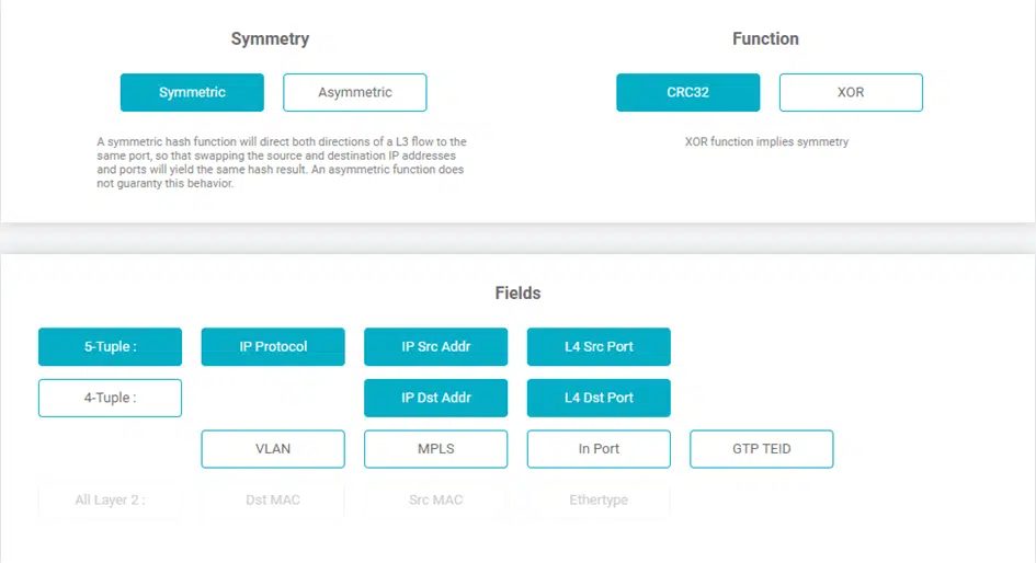
These hash values are determined using the so-called “5-tuple” mechanism, where each tuple represents a specific field in the header of each Ethernet frame. The available tuples on the Network Packet Broker (e.g. NEOXPacketLion), which are used for dynamic Load Balancing, are:
- Input Port (Physical Connection)
- Ethertype
- Source MAC
- Destination MAC
- VLAN Label
- MPLS Label
- GTP Tunnel Endpoint Identifier
- GTP Inner IP
- IP Protocol
- Source IP
- Destination IP
- Layer-4 Source PORT
- Layer-4 Destination PORT
Depending on the structure and setup of the network, and depending on whether packets are transported using NAT, another very common distribution of tuples is:
- IP Protocol
- Source IP
- Destination IP
- Layer-4 Source PORT
- Layer-4 Destination PORT
With “5-tuple” based Load Balancing, all the above-mentioned tuples are used to form a hash value which ensures that all packets, including the corresponding reverse direction, always leave the Network Packet Broker via the same port and thus, for example, the security system used always and fundamentally only receives complete sessions for evaluation.
Hash Values
In order to be able to generate the actual hash value on which the Load Balancing is based, the user has two different functions at his disposal, CRC32 and XOR.
By means of the CRC32 function, hash keys with a length of 32 bits can be generated and can be used both symmetrically and asymmetrically, while the XOR function creates a 16-bit long hash key, which, depending on the intended use, allows a higher-resolution distribution of the data, but can only output it symmetrically.
This symmetry means that even if the source IP and destination IP are swapped, as is known from regular Layer 3 conversations, the function still calculates the same hash key and thus the full Layer 3 conversations always leave the Network Packet Broker on the same physical port.
In the case of an asymmetric distribution, which is only supported by the CRC32 function, the Network Packet Broker PacketLion would calculate different hash values in the situation described above and thus also be output accordingly on different physical ports.
Dynamic Load Balancing
Another, additional function of Load Balancing is the possible dynamics with which this feature can be extended. In the case of dynamic Load Balancing, in addition to the hash value explained above, the percentage utilisation of each port that is part of the Load Balancing port group is also included in the calculation.
Of course, this procedure does not split any flows, and it also ensures that if a flow is issued based on the calculations on a specific port, this flow will always leave the Network Packet Broker via the same port in the future.
By means of a configurable timeout, the user can define when a flow loses its affiliation to an output port. In the event of a recurrence, this is then output to the participants of the load-balancing port group again in a regular manner and, both by detecting the load in the TX stream and by means of the hash value generation, it is determined which output port of the Network Packet Broker is currently most suitable for bringing the data to the connected analysis system.
Conclusion
It turns out that distributing the incoming data load by means of load balancing has been an effective way of utilising security, analysis and monitoring systems for many years. Over the years, this process has been further improved and culminates in the Dynamic Load Balancing that the PacketLion series has.
Constantly following up the configuration with regard to the distribution of the individual sessions to the connected systems is no longer necessary; this is now taken over by the intelligence of the Network Packet Broker and allows the user to use the full potential of his systems and avoid unnecessary expenditure.